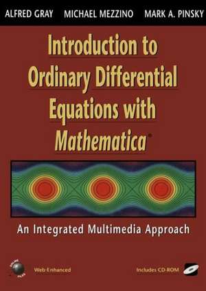
Introduction to Ordinary Differential Equations with Mathematica de Alfred Gray

Introduction to Ordinary Differential Equations with Mathematica: An Integrated Multimedia Approach

Alfred Gray

Michael Mezzino

Mark A. Pinsky

en Limba Engleză Paperback – 31 aug 2013

These materials - developed and thoroughly class tested over many years by the authors -are for use in courses at the sophomore/junior level. A prerequisite is the calculus of one variable, although calculus of several variables, and linear algebra are recommended. The text covers the standard topics in first and second order equations, power series solutions, first order systems, Laplace transforms, numerical methods and stability of non-linear systems. Liberal use is made of programs in Mathematica, both for symbolic computations and graphical displays. The programs are described in separate sections, as well as in the accompanying Mathematica notebooks. However, the book has been designed so that it can be read with or without Mathematica and no previous knowledge of Mathematica is required. The CD-ROM contains the Mathematica solution of worked examples, a selection of various Mathematica notebooks, Mathematica movies and sample labs for students. Mathematica programs and additional problem/example files will be available online through the TELOS Web site and the authors dedicated web site.

Citește tot Restrânge

Descriere

These materials, which have been developed and thoroughly class tested over a period of several years by the authors, are intended for use in courses in differential equations taught at the sophomore/junior level in American colleges and universities. Prerequisites for using these materials is the calculus of one variable, although calculus of several variables, and linear algrbra, are recommended. The text covers the standard topics in first and second order equations, power series solutions, first order systems, Laplace transforms, numerical methods and stability of non-linear systems. For historical completeness, the authors have also included the solution methods of Bernoulli, Clariaut, and Lagrange, if instructors wish to cover them. Liberal use is made of programs in Mathemtica, both for symbolic computations and graphical displays. The programs are described in separate sections, as well as in the accompanying Mathematica notebooks. The book has been designed so that it can be read with or without Mathematica and no pre-requisite knowledge of Mathematica is required to use the book, not to deal with the Mathematica programs contained in ODE.m, the special Mathematica software package residing on the CD-ROM accompanying the text. ODE.m enables students to solve differential equations, much as a calculator would. The CD-ROM, in addition to containing ODE.m, also contains the Mathematica solution of worked examples, the Mathematica solution of exercises, a protrait gallery of some 48 mathematicians who have contributed to the field of differential equations, a selction of various Mathematica noteboosk, Mathematica movies and sample labs for students. Mathematica programs and additional problem/example files will be made available online through the TELOS Web site (www.telospub.com) and the author's dedicated web site:

Cuprins

1. Basic Concepts.- 1.1 The Notion of a Differential Equation.- 1.2 Sources of Differential Equations.- 1.3 Solving Differential Equations.- 2. Using Mathematica.- 2.1 Getting Started with Mathematica Getting Started with Mathematica.- 2.2 Mathematica Notation versus Ordinary Mathematical Notation.- 2.3 Plotting in Mathematica.- 3. First-Order Differential Equations.- 3.1 Introduction to First-Order Equations.- 3.2 First-Order Linear Equations.- 3.3 Separable Equations.- 3.4 Exact Equations and Integrating Factors.- 3.5 Homogeneous First-Order Equations.- 3.6 Bernoulli Equations.- 4. The Package ODE • m.- 4.1 Getting Started with ODE.- 4.2 Features of ODE.- 4.3 Plotting with ODE.- 4.4 First-Order Linear Equations viaODE.- 4.5 Separable Equations via ODE.- 4.6 First-Order Equations with Integrating Factors via ODE.- 4.7 First-Order Homogeneous Equations viaODE.- 4.8 Bernoulli Equations via ODE.- 4.9 Clairaut and Lagrange Equations viaODE.- 4.10 Nonelementary Integrals.- 4.11 Using ODE to Define New Functions Ill.- 4.12 Riccati Equations.- 5. Existence and Uniqueness of Solutions of First-Order Differential Equations.- 5.1 The Existence and Uniqueness Theorem.- 5.2 Explosions and a Criterion for Global Existence.- 5.3 Picard Iteration.- 5.4 Proofs of Existence Theorems.- 5.5 Direction Fields and Differential Equations.- 5.6 Stability Analysis of Nonlinear First-Order Equations.- 6. Applications of First-Order Equations I.- 6.1 Population Models with Constant Growth Rate.- 6.2 Population Models with Variable Growth Rate.- 6.3 Logistic Model of Population Growth.- 6.4 Population Growth with Harvesting.- 6.5 Population Models for the United States.- 6.6 Temperature Equalization Models.- 7. Applications of First-Order Equations II.- 7.1 Application of First-Order Equations to Elementary Mechanics.- 7.2 Rocket Propulsion.- 7.3 Electrical Circuits.- 7.4 Mixing Problems.- 7.5 Pursuit Curves.- 8. Second-Order Linear Differential Equations.- 8.1 General Forms and Examples.- 8.2 Existence and Uniqueness Theory.- 8.3 Fundamental Sets of Solutions to the Homogeneous Equation.- 8.4 TheWronskian 2.- 8.5 Linear Independence and the Wronskian.- 8.6 Reduction of Order.- 8.7 Equations with Given Solutions.- 9. Second-Order Linear Differential Equations with Constant Coefficients.- 9.1 Constant-Coefficient Second-Order Homogeneous Equations.- 9.2 Complex Constant-Coefficient Second-Order Homogeneous Equations.- 9.3 The Method of Undetermined Coefficients.- 9.4 The Method of Variation of Parameters.- 10. Using ODE to Solve Second-Order Linear Differential Equations.- 10.1 Using ODE to Solve Second-Order Constant-Coefficient Equations.- 10.2 Details of ODE for Second-Order Constant-Coefficient Equations.- 10.3 Reduction of Order and Trial Solutions via ODE.- 10.4 Equations with Given Solutions via ODE.- 11. Applications of Linear Second-Order Equations 325.- 11.1 Mass-Spring Systems.- 11.2 Forced Vibrations of Mass-Spring Systems.- 11.3 Electrical Circuits.- 11.4 Sound.- 12. Higher-Order Linear Differential Equations.- 12.1 General Forms.- 12.2 Constant-Coefficient Higher-Order Homogeneous Equations.- 12.3 Variation of Parameters for Higher-Order Equations.- 12.4 Higher-Order Differential Equations via ODE.- 12.5 Seminumerical Solutions of Higher-Order Constant-Coefficient Equations.- 13. Numerical Solutions of Differential Equations.- 13.1 The Euler Method.- 13.2 The Heun Method.- 13.3 The Runge-Kutta Method.- 13.4 Solving Differential Equations Numerically with ODE.- 13.5 ODE’s Implementation of Numerical Methods.- 13.6 Using NDSolve.- 13.7 Adaptive Step Size and Error Control.- 13.8 The Numerov Method.- 14. The Laplace Transform.- 14.1 Definition and Properties of the Laplace Transform.- 14.2 Piecewise Continuous Functions.- 14.3 Using the Laplace Transform to Solve Initial Value Problems.- 14.4 The Gamma Function.- 14.5 Computation of Laplace Transforms.- 14.6 Step Functions.- 14.7 Second-Order Equations with Piecewise Continuous.- Forcing Functions.- 14.8 Impulse Functions.- 14.9 Convolution.- 14.10 Laplace Transforms via ODE.- 15. Systems of Linear Differential Equations.- 15.1 Notation and Definitions for Systems.- 15.2 Existence and Uniqueness Theorems for Systems.- 15.3 Solution of Upper Triangular Systems by Elimination.- 15.4 Homogeneous Linear Systems.- 15.5 Constant-Coefficient Homogeneous Systems.- 15.6 The Method of Undetermined Coefficients for Systems.- 15.7 The Method of Variation of Parameters for Systems.- 15.8 Solving Systems Using the Laplace Transform.- 16. Phase Portraits of Linear Systems.- 16.1 Phase Portraits of Two-Dimensional Linear Systems.- 16.2 Using ODE to Solve Linear Systems.- 16.3 Phase Portraits of Two-Dimensional Linear Systems via ODE.- 17. Stability of Nonlinear Systems.- 17.1 Curves.- 17.2 Autonomous Systems.- 17.3 Critical Points of Systems of Differential Equations.- 17.4 Stability and Asymptotic Stability of Nonlinear Systems.- 17.5 Stability by Linearized Approximation.- 17.6 Lyapunov Stability Theory.- 18. Applications of Linear Systems.- 18.1 Coupled Systems of Oscillators.- 18.2 Electrical Circuits.- 18.3 Markov Chains.- 19. Applications of Nonlinear Systems.- 19.1 Numerical Solutions of Systems of Differential Equations.- 19.2 Predator-Prey Modeling.- 19.3 The Van Der Pol Equation.- 19.4 The Simple Pendulum.- 19.5 The Fundamental Theorem of Plane Curves.- 20 Power Series Solutions of Second-Order Equations.- 20.1 Review of Power Series.- 20.2 Power Series via >Mathematica.- 20.3 Power Series Solutions about an Ordinary Point.- 20.4 The Airy Equation.- 20.5 The Legendre Equation.- 20.6 Convergence of Series Solutions.- 20.7 Series Solutions of Differential Equations Using ODE.- 21. Frobenius Solutions of Second-Order Equations.- 21.1 Solutions about a Regular Singular Point.- 21.2 The Cauchy-Euler Equation.- 21.3 Method of Frobenius: The First Solution.- 21.4 Bessel Functions I.- 21.5 Method of Frobenius: The Second Solution.- 21.6 Bessel Functions II.- 21.7 Bessel Functions via >Mathematica.- 21.8 An Aging Spring.- 21.9 The Hypergeometric Equation.- A. Appendix: Review of Linear Algebra and Matrix Theory.- A.l Vector and Matrix Notation.- A.2 Determinants and Inverses.- A.3 Systems of Linear Equations and Determinants.- A.4 Eigenvalues and Eigenvectors.- A.5 The Exponential of a Matrix.- A.6 Abstract Vector Spaces.- A.7 Vectors and Matrices with Mathematica.- A.8 Solving Equations with Mathematica.- A.9 Eigenvalues and Eigenvectors with Mathematica.- B. Appendix: Systems of Units.- Answers.- General Index.- Name Index.