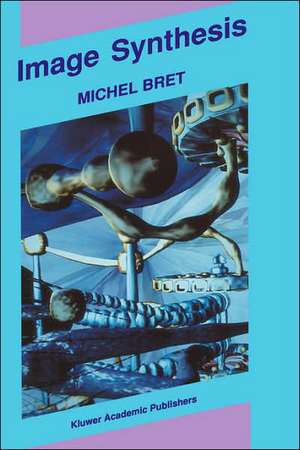
Image Synthesis
Autor Michel Breten Limba Engleză Hardback – 29 noi 1991
| Toate formatele și edițiile | Preț | Express |
|---|---|---|
| Paperback (1) | 822.00 lei 38-44 zile | |
| SPRINGER NETHERLANDS – 20 sep 2012 | 822.00 lei 38-44 zile | |
| Hardback (1) | 1030.47 lei 38-44 zile | |
| SPRINGER NETHERLANDS – 29 noi 1991 | 1030.47 lei 38-44 zile |
Preț: 1030.47 lei
Preț vechi: 1288.09 lei
-20% Nou
Puncte Express: 1546
Preț estimativ în valută:
197.20€ • 214.13$ • 165.65£
197.20€ • 214.13$ • 165.65£
Carte tipărită la comandă
Livrare economică 18-24 aprilie
Preluare comenzi: 021 569.72.76
Specificații
ISBN-13: 9780792314882
ISBN-10: 0792314883
Pagini: 289
Dimensiuni: 155 x 235 x 19 mm
Greutate: 0.61 kg
Ediția:1992
Editura: SPRINGER NETHERLANDS
Colecția Springer
Locul publicării:Dordrecht, Netherlands
ISBN-10: 0792314883
Pagini: 289
Dimensiuni: 155 x 235 x 19 mm
Greutate: 0.61 kg
Ediția:1992
Editura: SPRINGER NETHERLANDS
Colecția Springer
Locul publicării:Dordrecht, Netherlands
V-ar putea interesa
-
 Passive Imaging with Ambient NoiseJosselin Garnier-20%Preț: 838.30 lei1047.88 lei
 -
 -9%Preț: 865.41 lei951.00 lei
 -
 -9%Preț: 720.98 lei792.29 lei
 -
 Acoustical Sensing and ImagingHua Lee-25%Preț: 495.78 lei664.93 lei
 -
 An Introduction to 3D PrintingVictoria ZukasPreț: 338.89 lei
 -
 -15%Preț: 661.97 lei778.80 lei
 -
 -15%Preț: 658.22 lei774.39 lei
 -
 Dense Image Correspondences for Computer VisionTal Hassner-15%Preț: 647.27 lei761.49 lei
 -
 Image Processing and Communications Challenges 7Ryszard S. Choraś-20%Preț: 988.32 lei1235.41 lei
 -
 Art and IllusionistsNicholas WadePreț: 344.42 lei
 -
 Advances in Face Detection and Facial Image AnalysisMichal KawulokPreț: 404.29 lei
 -
 Preț: 374.68 lei
 -
 -20%Preț: 659.51 lei824.38 lei
 -
 Preț: 393.35 lei
 -
 Hyperspectral Image ProcessingLiguo Wang-15%Preț: 653.98 lei769.39 lei
 -
 -20%Preț: 1294.36 lei1617.95 lei
 -
 -20%Preț: 1294.55 lei1618.19 lei
 -
 Wireless Networked Music PerformanceLeonardo GabrielliPreț: 378.34 lei
 -
 Bayesian Methods in the Search for MH370Neil GordonPreț: 174.24 lei
Public țintă
ResearchDescriere
The
images
produced
by
means
ofcomputers
have
invaded
our
daily
lives.
One
has
but
to
see
the
"identification
logos"
of
most
television
broadcasts
or
some
advenisement
"spots"
to
be
convinced
of
this.
This
proves
that
the
synthesis
ofimages
has
reached
maturity.
The
progress
that
has
been
made
in
the
last
few
years
allows
one
to
predict
the
use
ofrealistic
illustrations
in
more
and
more
domains
ofapplication.
It
is
thus
understandable
that
more
and
more
people
seek
to
understand
how
these
images
are
produced.
Such
a
person
may
be
an
amateur
who
likes
to
understand
in
a
general
way
the
processing
involved,
or
he
may
be
a
computer
scientist
who
wants
to
develop
some
new
application
using
graphics
procedures.
This
book
by
Michel
Bret
meets
these
desires
by
giving
a
complete
overview
of
the
techniques
of
image
synthesis
by
computer.
The
different
stages
of
the
creation
of
a
numerical
image
are
explained
in
detail,
and
they
are
accompanied
by
descriptions
of
the
most
modem
methods.
Thus
the
geometrical
models
that
are
described
go
from
those
with
plane
polygonal
facets,
via
surfaces
of
all
types,
to
systems
of
panicles.
Visualization
is
treated
in
complete
detail,
and
due
attention
is
given
to
all
the
various
roads
that
lead
to
a
realistic
image:
simple
projections
on
the
basis
of
wire-frame
models,
the
elimination
of
hidden
pans,
and
fmally
the
modelling
oflight
and
its
effects.
Cuprins
1.
Images.-
1.1.
Images
and
communication.-
1.1.1.
Speaking.-
1.1.2.
Writing.-
1.1.3.
Images.-
1.1.4.
Discourse,
image,
and
computer.-
1.2.
Visual
perception.-
1.2.1.
Thought
and
vision.-
1.2.2.
The
mechanisms
of
photoreception.-
1.2.3.
The
optical
paths.-
1.2.4.
The
treatment
of
visual
information.-
1.2.5.
Multiplexing
of
sensorial
messages.-
1.3.
Different
aspects
of
images.-
1.3.1.
Attempt
to
define
the
concept
of
an
image.-
1.3.2.
Physical
images.-
1.3.3.
Psychic
images.-
1.3.4.
The
particular
status
of
numerical
images.-
2.
Numerical
images.-
2.1.
Image
and
computer.-
2.1.1.
Images
as
memory.-
2.1.1.1.
Psychic
images
and
memory.-
2.1.1.2.
Encoding
and
decoding
of
images.-
2.1.2.
Representations.-
2.1.2.1.
Analogue
representation.-
2.1.2.2.
Numerical
representation.-
2.1.3.
Numerical
(digital)
images.-
2.1.3.1.
Screen
memory.-
2.1.3.2.
Vector
memory.-
2.2.
The
graphical
peripherals.-
2.2.1.
Central
unit
and
peripherals.-
2.2.2.
Graphical
output
peripherals.-
2.2.2.1.
History.-
2.2.2.2.
Printers,
tape
and
card
punchers.-
2.2.2.3.
Plotters.-
2.2.2.4.
Cathode
ray
tubes.-
2.2.2.5.
COMs.-
2.2.2.6.
Flat
screens.-
2.2.2.7.
Laser
techniques.-
2.2.3.
Peripherals
of
graphics
processing.-
2.2.3.1.
The
optical
pen.-
2.2.3.2.
Data
tablet.-
2.2.3.3.
Mouse.-
2.2.3.4.
Digitizers
of
images.-
2.2.3.5.
Others.-
2.2.4.
Interaction.-
2.3.
Cathode
ray
tubes.-
2.3.1.
History.-
2.3.2.
Principles
of
functioning.-
2.3.3.
Scanning
modes.-
2.3.4.
Graphics
processor.-
2.3.5.
Tubes
with
free
scanning.-
2.3.6.
Tubes
with
memory
(or
with
image
preservation).-
2.3.7.
Tubes
with
recurrent
scanning.-
2.3.8.
Color
screens.-
2.3.9.
Linearization
of
the
intensity
levels.-
2.3.10.
Look
up
tables.-
2.3.10.1.
Principle.-
2.3.10.2.
Applications.-
2.3.10.3.
Digitizers
of
images.-
2.4.
Flat
screens.-
2.5.
The
programming
of
graphics
processors.-
3.
Modelling
problems.-
3.1.
Image
and
formalism.-
3.1.1.
Image
and
model.-
3.1.2.
The
computer
as
a
tool
of
creation.-
3.1.3.
The
different
levels
of
description.-
3.2.
The
modelling
of
images.-
3.2.1.
Processing
of
a
numerical
image.-
3.2.2.
Synthesis.-
3.2.3.
Abstract
plane
images.-
3.2.4.
Figurative
plane
images.-
3.2.5.
Three-dimensional
images.-
3.2.6.
Realistic
images.-
3.3.
Constructive
geometry.-
3.3.1.
Modular
structures.-
3.3.2.
Euler
operators.-
3.3.3.
Applications.-
3.4.
Polyhedral
models.-
3.4.1.
Polyhedral
approximation
of
a
curved
surface.-
3.4.1.1.
Modelling
by
means
of
facets.-
3.4.1.2.
Triangulation
methods.-
3.4.2.
Data
structures
associated
with
polyhedral
descriptions.-
3.4.3.
Domains
of
applications.-
3.5.
Curves
and
surfaces.-
3.5.1.
Graphical
primitives.-
3.5.2.
Generating
plane
curves.-
3.5.2.1.
Polygonal
approximations.-
3.5.2.2.
Reduction
of
numerical
plane
curves.-
3.5.3.
Parametic
curves
and
surfaces.-
3.5.3.1.
Cubics.-
3.5.3.2.
Coons’
surfaces.-
3.5.3.3.
Bezier
curves
and
surfaces.-
3.5.3.4.
B-spline
curves
and
surfaces.-
3.5.3.5.
Beta-splines.-
3.5.4.
The
visualization
of
curves
and
surfaces.-
3.6.
Fractal
objects.-
3.6.1.
Fractal
objects
according
to
Benoit
Mandelbrot.-
3.6.1.1.
Continuity
and
reality.-
3.6.1.2.
The
concept
of
dimension.-
3.6.1.3.
Measure.-
3.6.1.4.
The
concept
of
an
internal
homothety.-
3.6.1.5.
Homothety
dimension.-
3.6.1.6.
Stochastic
models.-
3.6.1.7.
Terrain
models.-
3.6.2.
Algorithms
for
the
generation
of
three-dimensional
fractal
objects.-
3.6.2.1.
Numerical
images
and
fractal
dimension.-
3.6.2.2.
Iteration
of
functions.-
3.6.2.3.
Stochastic
models.-
3.6.2.4.
Stochastic
primitives.-
3.6.2.5.
Stochastic
movement.-
3.7.
Systems
of
particles.-
3.7.1.
The
modeling
of
unsharp
objects.-
3.7.2.
Systems
of
particles.-
3.7.3.
Application
to
the
modelling
of
fire
and
explosions.-
3.8.
Modelling
waves.-
3.8.1.
Explanation
of
the
problem.-
3.8.2.
Peachey’s
model.-
3.8.3.
The
model
of
Fournier
and
Reeves.-
3.9.
The
synthesis
of
fabrics.-
3.9.1.
Explanation
of
the
problem.-
3.9.2.
Weil’s
model.-
3.9.2.1.
The
conditions.-
3.9.2.2.
Approximation
of
the
surface.-
3.9.2.3.
Iterative
approximation.-
3.10.
The
modelling
of
shells
and
plants.-
3.10.1.
Explanation
of
the
problem.-
3.10.2.
Kawaguchi
and
the
sea.-
3.10.3.
Plants
and
formal
languages.-
3.10.4.
Tree-like
models
of
plants.-
3.10.5.
AMAP.-
4.
Problems
of
visualization.-
4.1.
The
visualization
of
numerical
images.-
4.1.1.
Numerical
images.-
4.1.2.
Coding
numerical
images.-
4.1.2.1.
Run-length
coding.-
4.1.2.2.
Coding
according
to
Freeman.-
4.1.2.3.
Coding
by
means
of
quaternary
trees.-
4.2.
2D-images.-
4.2.1.
Graphical
primitives.-
4.2.1.1.
Points.-
4.2.1.2.
Segments.-
4.2.1.3.
Simple
figures.-
4.2.2.
2D
clipping.-
4.2.2.1.
Explanation
of
the
problem.-
4.2.2.2.
Clipping
of
a
segment
by
a
rectangular
window.-
4.2.2.3.
Clipping
by
an
arbitrary
window.-
4.2.2.4.
The
clipping
of
polygons.-
4.2.2.5.
Concave
windows.-
4.2.3.
Colouring
surfaces.-
4.2.3.1.
Explanation
of
the
problem.-
4.2.3.2.
Algorithms
which
work
on
the
image
memory.-
4.2.3.3.
Algorithms
which
use
associated
data
structures.-
4.2.4.
The
use
of
smoothing.-
4.2.4.1.
Principles.-
4.2.4.2.
Smoothings
defined
on
the
basis
of
poles.-
4.2.4.3.
Methods
of
colour
points.-
4.3.
Perspective
projections.-
4.3.1.
3D-Images.-
4.3.1.1.
Object
space
and
image
space.-
4.3.1.2.
The
perception
of
space.-
4.3.1.3.
Perspective
projection.-
4.3.1.4.
The
problem
of
entering
the
data.-
4.3.2.
Homogeneous
coordinates.-
4.3.3.
The
matrix
associated
to
a
linear
transformation.-
4.3.3.1.
Matrix
of
a
linear
transformation.-
4.3.3.2.
Product
of
linear
transformations.-
4.3.3.3.
Examples.-
4.3.4.
Perspective
transformations.-
4.3.5.
Clipping.-
4.3.6.
Coordinate
system
of
the
screen
and
perspective
projection.-
4.4.
Aliasing.-
4.4.1.
Explanation
of
the
problem.-
4.4.2.
Filtering
a
numerical
image.-
4.4.3.
Increasing
the
resolution.-
4.4.4.
Random
sampling.-
4.4.5.
The
method
of
dividing
pixels.-
4.5.
Motifs,
mappings.-
4.5.1.
Explanation
of
the
problem.-
4.5.2.
Motifs.-
4.5.3.
Maps.-
4.6.
Textures.-
4.6.1.
Definition
of
the
concept
of
texture.-
4.6.2.
Analysis
and
synthesis
of
textures.-
4.6.3.
Blinn’s
method.-
4.6.4.
3D-textures.-
5.
The
elimination
of
hidden
parts.-
5.1.
The
problem
of
hidden
parts.-
5.1.1.
Explanation
of
the
problem.-
5.1.2.
Principles.-
5.2.
Elements
of
geometry.-
5.2.1.
Box
tests.-
5.2.2.
Belonging
to
the
interior
of
a
polygon.-
5.2.3.
Equations
of
planes.-
5.2.4.
Sorting
problems.-
5.2.5.
Coherence.-
5.3.
Classification
of
algorithms.-
5.4.
The
algorithm
with
a
mobile
horizon.-
5.4.1.
Principles.-
5.4.2.
The
algorithm.-
5.4.3.
Implementation.-
5.5.
Roberts’
algorithm.-
5.5.1.
Principles.-
5.5.2.
Elimination
of
back
facets.-
5.5.3.
Elimination
of
the
remaining
edges.-
5.6.
Schumacker’s
algorithm.-
5.7.
The
algorithm
of
Newell-Newell-Sancha.-
5.7.1.
Principles.-
5.7.2.
Newell’s
algorithm.-
5.8.
Warnock’s
algorithm.-
5.8.1.
Principles.-
5.8.2.
Optimization.-
5.9.
Scan-line
algorithms.-
5.10.
Application
of
automatic
programming:
Goad’salgorithm.-
5.11.
Using
coherence.-
5.12.
The
z-buffer
algorithm.-
5.12.1.
Principles.-
5.12.2.
Implementation.-
5.12.3.
Limitations
of
the
method.-
5.12.4.
Scan-line
and
z-buffer.-
5.13.
The
ray-tracing
algorithm.-
5.13.1.
Principles.-
5.13.2.
Implementation.-
5.13.3.
Calculating
intersections.-
5.13.4.
Arranging
the
objects
in
a
hierarchy.-
6.
Illumination
models.-
6.1.
Illumination
of
a
scene.-
6.2.
The
models
of
Phong
and
of
Blinn.-
6.2.1.
Diffuse
illumination
(or
ambient
lighting).-
6.2.2.
Lambert’s
law.-
6.2.3.
Specular
reflection.-
6.2.4.
Multiple
sources.-
6.3.
Cook’s
model.-
6.3.1.
The
model.-
6.3.2.
Bidirectional
distribution
of
reflected
light.-
6.3.3.
Spectral
distribution
of
reflected
light.-
6.4.
Transparency.-
6.5.
Smoothing
methods.-
6.5.1.
The
smoothing
problem.-
6.5.2.
Gouraud
smoothing.-
6.5.3.
Phong
smoothing.-
6.5.4.
Comparison
of
the
two
methods.-
6.6.
Shadows.-
6.6.1.
Explanation
of
the
problem.-
6.6.2.
Projection
method.-
6.6.3.
z-buffer
method.-
6.6.4.
Ray-tracing
method.-
6.7.
Radiosity.-
6.7.1.
The
illumination
problem.-
6.7.2.
The
radiosity
principle.-
6.7.3.
Calculation
of
the
form
coefficients.-
6.7.4.
Cohen’s
hemi-cube.-
6.8.
Ray-tracing.-
6.8.1.
Principles.-
6.8.2.
Whitted’s
model.-
6.8.3.
Calculating
secondary
rays.-
6.8.4.
Anti-aliasing.-
6.8.5.
Optimization.-
6.8.5.1.
Box
tests.-
6.8.5.2.
Optimization
according
to
the
type
of
primitives.-
6.8.6.
Bundle
tracing.-
6.8.6.1.
Ray
and
bundle.-
6.8.6.2.
Representation
of
a
ray
in
a
bundle.-
6.8.6.3.
Matrices
associated
to
optical
systems.-
6.8.6.4.
Evaluation
of
the
deviation.-
6.9.
Simulation
of
clouds
and
fluffy
surfaces.-
6.9.1.
Dispersion
models
in
a
cloud.-
6.9.2.
Phase
functions.-
6.10.
Simulation
of
atmospheric
dispersion.-
6.10.1.
Explanation
of
the
problem.-
6.10.2.
Nishita’s
model.