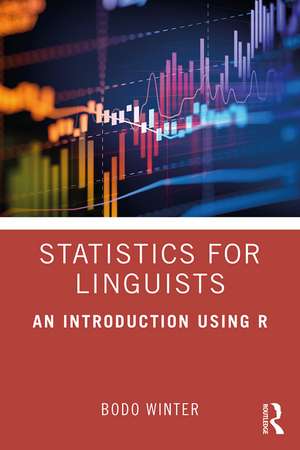
Statistics for Linguists: An Introduction Using R
Autor Bodo Winteren Limba Engleză Paperback – 13 noi 2019
| Toate formatele și edițiile | Preț | Express |
|---|---|---|
| Paperback (1) | 342.06 lei 6-8 săpt. | |
| Taylor & Francis – 13 noi 2019 | 342.06 lei 6-8 săpt. | |
| Hardback (1) | 766.16 lei 6-8 săpt. | |
| Taylor & Francis – 14 noi 2019 | 766.16 lei 6-8 săpt. |
Preț: 342.06 lei
Nou
Puncte Express: 513
Preț estimativ în valută:
65.45€ • 68.52$ • 54.16£
65.45€ • 68.52$ • 54.16£
Carte tipărită la comandă
Livrare economică 05-19 aprilie
Preluare comenzi: 021 569.72.76
Specificații
ISBN-13: 9781138056091
ISBN-10: 113805609X
Pagini: 326
Ilustrații: 65 Line drawings, black and white
Dimensiuni: 152 x 229 x 25 mm
Greutate: 0.5 kg
Ediția:1
Editura: Taylor & Francis
Colecția Routledge
Locul publicării:Oxford, United Kingdom
ISBN-10: 113805609X
Pagini: 326
Ilustrații: 65 Line drawings, black and white
Dimensiuni: 152 x 229 x 25 mm
Greutate: 0.5 kg
Ediția:1
Editura: Taylor & Francis
Colecția Routledge
Locul publicării:Oxford, United Kingdom
Public țintă
Postgraduate and UndergraduateCuprins
Table of contents
0. Preface: Approach and how to use this book
0.1. Strategy of the book
0.2. Why R?
0.3. Why the tidyverse?
0.4. R packages required for this book
0.5. What this book is not
0.6. How to use this book
0.7. Information for teachers
1. Introduction to base R
1.1. Introduction
1.2. Baby steps: simple math with R
1.3. Your first R script
1.4. Assigning variables
1.5. Numeric vectors
1.6. Indexing
1.7. Logical vectors
1.8. Character vectors
1.9. Factor vectors
1.10. Data frames
1.11. Loading in files
1.12. Plotting
1.13. Installing, loading, and citing packages
1.14. Seeking help
1.15. A note on keyboard shortcuts
1.16. Your R journey: The road ahead
2. Tidy functions and reproducible R workflows
2.1. Introduction
2.2. tibble and readr
2.3. dplyr
2.4. ggplot2
2.5. Piping with magrittr
2.6. A more extensive example: iconicity and the senses
2.7. R markdown
2.8. Folder structure for analysis projects
2.9. Readme files and more markdown
2.10. Open and reproducible research
3. Models and distributions
3.1. Models
3.2. Distributions
3.3. The normal distribution
3.4. Thinking of the mean as a model
3.5. Other summary statistics: median and range
3.6. Boxplots and the interquartile range
3.7. Summary statistics in R
3.8. Exploring the emotional valence ratings
3.9. Chapter conclusions
4. Introduction to the linear model: Simple linear regression
4.1. Word frequency effects
4.2. Intercepts and slopes
4.3. Fitted values and residuals
4.4. Assumptions: Normality and constant variance
4.5. Measuring model fit with
4.6. A simple linear model in R
4.7. Linear models with tidyverse functions
4.8. Model formula notation: Intercept placeholders
4.9. Chapter conclusions
5. Correlation, linear, and nonlinear transformations
5.1. Centering
5.2. Standardizing
5.3. Correlation
5.4. Using logarithms to describe magnitudes
5.5. Example: Response durations and word frequency
5.6. Centering and standardization in R
5.7. Terminological note on the term ‘normalizing’
5.8. Chapter conclusions
6. Multiple regression
6.1. Regression with more than one predictor
6.2. Multiple regression with standardized coefficients
6.3. Assessing assumptions
6.4. Collinearity
6.5. Adjusted
6.6. Chapter conclusions
7. Categorical predictors
7.1. Introduction
7.2. Modeling the emotional valence of taste and smell words
7.3. Processing the taste and smell data
7.4. Treatment coding in R
7.5. Doing dummy coding ‘by hand’
7.6. Changing the reference level
7.7. Sum coding in R
7.8. Categorical predictors with more than two levels
7.9. Assumptions again
7.10. Other coding schemes
7.11. Chapter conclusions
8. Interactions and nonlinear effects
8.1. Introduction
8.2. Categorical * continuous interactions
8.3. Categorical * categorical interactions
8.4. Continuous * continuous interactions
8.5. Continuous interactions and regression planes
8.6. Higher-order interactions
8.7. Chapter conclusions
9. Inferential statistics 1: Significance testing
9.1. Introduction
9.2. Effect size: Cohen’s
9.3. Cohen’s in R
9.4. Standard errors and confidence intervals
9.5. Null hypotheses
9.6. Using to measure the incompatibility with the null hypothesis
9.7. Using the -distribution to compute -values
9.8. Chapter conclusions
10. Inferential statistics 2: Issues in significance testing
10.1. Common misinterpretations of -values
10.2. Statistical power and Type I, II, M, and S errors
10.3. Multiple testing
10.4. Stopping rules
10.5. Chapter conclusions
11. Inferential statistics 3: Significance testing in a regression context
11.1. Introduction
11.2. Standard errors and confidence intervals for regression coefficients
11.3. Significance tests with multi-level categorical predictors
11.4. Another example: the absolute valence of taste and smell words
11.5. Communicating uncertainty for categorical predictors
11.6. Communicating uncertainty for continuous predictors
11.7. Chapter conclusions
12. Generalized linear models: Logistic regression
12.1. Motivating generalized linear models
12.2. Theoretical background: Data-generating processes
12.3. The log odd function and interpreting logits
12.4. Speech errors and blood alcohol concentration
12.5. Predicting the dative alternation
12.6. Analyzing gesture perception: Hassemer & Winter (2016)
12.6.1. Exploring the dataset
12.6.2. Logistic regression analysis
12.7. Chapter conclusions
13. Generalized linear models 2: Poisson regression
13.1. Motivating Poisson regression
13.2. The Poisson distribution
13.3. Analyzing linguistic diversity using Poisson regression
13.4. Adding exposure variables
13.5. Negative binomial regression for overdispersed count data
13.6. Overview and summary of the generalized linear model framework
13.7. Chapter conclusions
14. Mixed models 1: Conceptual introduction
14.1. Introduction
14.2. The independence assumption
14.3. Dealing with non-independence via experimental design and averaging
14.4. Mixed models: Varying intercepts and varying slopes
14.5. More on varying intercepts and varying slopes
14.6. Interpreting random effects and random effect correlations
14.7. Specifying mixed effects models: lme4 syntax
14.8. Reasoning about your mixed model: The importance of varying slopes
14.9. Chapter conclusions
15. Mixed models 2: Extended example, significance testing, convergence issues
15.1. Introduction
15.2. Simulating vowel durations for a mixed model analysis
15.3. Analyzing the simulated vowel durations with mixed models
15.4. Extracting information out of lme4 objects
15.5. Messing up the model
15.6. Likelihood ratio tests
15.7. Remaining issues
15.7.1. -squared for mixed models
15.7.2. Predictions from mixed models
15.7.3. Convergence issues
15.8. Mixed logistic regression: Ugly selfies
15.9. Shrinkage and individual differences
15.10. Chapter conclusions
16. Outlook and strategies for model building
16.1. What you have learned so far
16.2. Model choice
16.3. The cookbook approach
16.4. Stepwise regression
16.5. A plea for subjective and theory-driven statistical modeling
16.6. Reproducible research
16.7. Closing words
References
Appendix A. Correspondences between significance tests and linear models
Appendix B. Reading recommendations
Notă biografică
Bodo Winter is Lecturer in Cognitive Linguistics in the Department of English Language and Applied Linguistics at the University of Birmingham, UK.
Descriere
This is the first statistics textbook on linear models for linguistics. The book covers simple uses of linear models through generalized models to more advanced approaches, maintaining its focus on conceptual issues and avoiding excessive mathematical details. It contains many applied examples using the R statistical programming environment.
